Programming with Python

Analyzing Temperature Data

While a lot of powerful tools are built into languages like Python, even more tools exist in libraries.

In order to load our temperature data, we need to import a library called NumPy. You should use this library if you want to do fancy things with numbers, especially if you have matrices or arrays. We can load NumPy using:

import numpy

Importing a library is like getting a piece of lab equipment out of a storage locker and setting it up on the bench. Libraries provide additional functionality to the basic Python packages, much like a new piece of equipment adds functionality to a lab space. Once we’ve loaded the library, we can use a tool in that library to read the data file:

numpy.loadtxt(fname='data/temperature.csv', delimiter=',')

array([[ 264.,  264.,  264., ...,  263.,  263.,  264.],
       [ 263.,  264.,  264., ...,  262.,  262.,  263.],
       [ 301.,  302.,  302., ...,  301.,  301.,  301.],
       [ 292.,  293.,  293., ...,  291.,  292.,  292.]])

The expression numpy.loadtxt(...) is a function call that asks Python to run the function loadtxt that belongs to the numpy library. This dotted notation is used everywhere in Python to refer to parts of things, with the syntax thing.component.

The function call to numpy.loadtxt has two parameters: the name of the file we want to read, and the delimiter that separates values on a line. These both need to be character strings (or strings for short), so we put them in quotes.

When we press Shift+Enter, the notebook runs our command. Since we haven’t told it what to do with the function’s output, the notebook displays it. In this case, that output is the data we just loaded. By default, only a few rows and columns are shown (with ... to omit elements when displaying big arrays). To save space, Python displays numbers as 1. instead of 1.0 when there’s nothing interesting after the decimal point.

Our call to numpy.loadtxt read our file but didn’t save the data in memory. To do that, we need to assign the array to a variable. A variable is just a name for a value, such as x, current_temperature, or subject_id. Python’s variables must begin with a letter and are case sensitive. We can create a new variable by assigning a value to it using =. As an illustration, let’s step back and instead of using a table of data, consider the simplest “collection” of data: a single value. The line below assigns the value 55 to a variable weight_kg:

weight_kg = 55

Once a variable has a value, we can print it to the screen:

print weight_kg

55

and do arithmetic with it:

print 'weight in pounds:', 2.2 * weight_kg

weight in pounds: 121.0

We can also change a variable’s value by assigning it a new one:

weight_kg = 57.5
print 'weight in kilograms is now:', weight_kg

weight in kilograms is now: 57.5

As the example above shows, we can print several things at once by separating them with commas.

If we imagine the variable as a sticky note with a name written on it, assignment is like putting the sticky note on a particular value:

Variables as Sticky Notes

This means that assigning a value to one variable does not change the values of other variables. For example, let’s store the subject’s weight in pounds in a variable:

weight_lb = 2.2 * weight_kg
print 'weight in kilograms:', weight_kg, 'and in pounds:', weight_lb

weight in kilograms: 57.5 and in pounds: 126.5

Creating Another Variable

and then change weight_kg:

weight_kg = 100.0
print 'weight in kilograms is now:', weight_kg, 'and weight in pounds is still:', weight_lb

weight in kilograms is now: 100.0 and weight in pounds is still: 126.5

Updating a Variable

Since weight_lb doesn’t “remember” where its value came from, it isn’t automatically updated when weight_kg changes. This is different from the way spreadsheets work.

Just as we can assign a single value to a variable, we can also assign an array of values to a variable using the same syntax. Let’s re-run numpy.loadtxt and save its result:

data = numpy.loadtxt(fname='data/temperature.csv',delimiter=',')

This statement doesn’t produce any output because an assignment doesn’t display anything. If we want to check that our data has been loaded, we can print the variable’s value:

print data

[[ 264.  264.  264. ...,  263.  263.  264.]
 [ 263.  264.  264. ...,  262.  262.  263.]
 [ 301.  302.  302. ...,  301.  301.  301.]
 [ 292.  293.  293. ...,  291.  292.  292.]]

Now that our data is in memory, we can start doing things with it. First, let’s ask what type of thing data refers to:

print type(data)

<class 'numpy.ndarray'>

The output tells us that the variable name data currently refers to an N-dimensional array created by the NumPy library. These data are daily average temperature normals (averages of three decades) for four stations around Flagstaff, AZ. We can see what its shape is like this:

print data.shape

(4, 365)

This tells us that data has 4 rows and 365 columns. When we created the variable data to store the temperature data, we didn’t just create the array. We also created information about the array, called members or attributes. This extra information describes data in the same way an adjective describes a noun. data.shape is an attribute of data which described the dimensions of data. We use the same dotted notation for the attributes of variables that we use for the functions in libraries because they have the same part-and-whole relationship.

If we want to get a single number from the array, we must provide an index in square brackets:

print 'first value in data:', data[0, 0]

first value in data: 264.0

print 'middle value in data:', data[2, 180]

middle value in data: 696.0

When referring to a two dimensional array, indices are numbered as row,column. The expression data[2, 180] may not surprise you, but data[0, 0] might. Programming languages like Fortran and MATLAB start counting at 1 because that’s what human beings have done for thousands of years. Languages in the C family (including C++, Java, Perl, and Python) count from 0 because that’s simpler for computers to do. As a result, if we have an M×N array in Python, its indices go from 0 to M-1 on the first axis and 0 to N-1 on the second. It takes a bit of getting used to, but one way to remember the rule is that the index is how many steps we have to take from the start to get the item we want.

mass = 47.5
age = 122
mass = mass * 2.0
age = age - 20

first, second = 'Grace', 'Hopper'
third, fourth = second, first
print third, fourth

Slicing

An index like [2, 180] selects a single element of an array, but we can select whole sections as well. For example, we can select the first ten days (columns) of values for the first two stations (rows) like this:

print data[0:2, 0:10]

[[ 264.  264.  264.  265.  265.  266.  266.  266.  267.  267.]
 [ 263.  264.  264.  265.  265.  266.  266.  267.  267.  268.]]

The slice 0:2 means, “Start at index 0 and go up to, but not including, index 2.” Again, the up-to-but-not-including takes a bit of getting used to, but the rule is that the difference between the upper and lower bounds is the number of values in the slice.

We don’t have to start slices at 0:

print data[2:4, 0:10]

[[ 301.  302.  302.  302.  303.  303.  304.  304.  305.  306.]
 [ 292.  293.  293.  294.  294.  295.  295.  296.  296.  297.]]

We also don’t have to include the upper and lower bound on the slice. If we don’t include the lower bound, Python uses 0 by default; if we don’t include the upper, the slice runs to the end of the axis, and if we don’t include either (i.e., if we just use ‘:’ on its own), the slice includes everything:

small = data[:2,360:]
print 'small is:'
print small

small is:
[[ 263.  263.  263.  263.  264.]
 [ 261.  261.  262.  262.  263.]]

Arrays also know how to handle common mathematical operations on their values. The simplest operations with data are arithmetic: add, subtract, multiply, and divide. When you do such operations on arrays, the operation is done on each individual element of the array. Thus:

doubledata = data * 2.0

will create a new array doubledata whose elements have the value of two times the value of the corresponding elements in data:

print 'original:'
print data[:2,360:]
print 'doubledata:'
print doubledata[:2,360:]

original:
[[ 263.  263.  263.  263.  264.]
 [ 261.  261.  262.  262.  263.]]
doubledata:
[[ 526.  526.  526.  526.  528.]
 [ 522.  522.  524.  524.  526.]]

If, instead of taking an array and doing arithmetic with a single value (as above) you did the arithmetic operation with another array of the same shape, the operation will be done on corresponding elements of the two arrays. Thus:

tripledata = doubledata + data

will give you an array where tripledata[0,0] will equal doubledata[0,0] plus data[0,0], and so on for all other elements of the arrays.

print 'tripledata:'
print tripledata[:2,360:]

tripledata:
[[ 789.  789.  789.  789.  792.]
 [ 783.  783.  786.  786.  789.]]

Arrays also know how to do more complex operations on their values. If we want to find the average temperature on all days across all stations, for example, we can just ask the array for its mean value

print data.mean()

457.837671233

mean is a method of the array, i.e., a function that belongs to it in the same way that the member shape does. If variables are nouns, methods are adjectives: they are some intrinsic characteristic of the object. We need empty parentheses for data.mean() even when we’re not passing in any parameters to tell Python to go and do something for us. data.shape doesn’t need () because it is just a description of the object but data.mean() requires the () because something has to be done with the object to find it.

NumPy arrays have lots of useful methods:

print 'maximum temperature:', data.max()
print 'minimum temperature:', data.min()
print 'standard deviation:', data.std()

maximum temperature: 714.0
minimum temperature: 261.0
standard deviation: 133.797538033

When analyzing data, though, we often want to look at partial statistics such as the maximum temperature value per station or the average temperature value per day across all stations. One way to do this is to create a new temporary array of the data we want, and then ask it to do the calculation:

station_0 = data[0, :] # 0 on the first axis, everything on the second
print 'maximum temperature for station 0:', station_0.max()

maximum temperature for station 0: 641.0

We don’t actually need to store the row in a variable of its own before calculating its statistics. Instead, we can combine the selection and the method call:

print 'maximum temperature for station 2:', data[2, :].max()

maximum temperature for station 2: 714.0

If we need the maximum temperature for every station or the average for each day for a single station, we can perform the operation across an axis. For this, most array methods allow us to specify the axis we want to work on. If we ask for the average across axis 0 (rows in our 2D example), we get:

print data.mean(axis=0)

[ 280.    280.75  280.75  281.5   281.75  282.5   282.75  283.25  283.75
  284.5   284.75  285.5   286.    286.75  287.    287.5   288.25  288.75
  289.25  290.    290.5   290.75  291.75  292.    292.75  293.5   294.
  295.    295.75  296.25  297.    298.25  298.75  299.75  300.75  301.75
  302.5   303.75  305.    306.    307.5   309.    310.5   311.75  313.25
  314.75  316.5   318.    319.75  321.25  323.    325.    326.5   328.25
  330.25  332.    334.    335.75  337.5   339.5   341.25  343.25  345.25
  347.25  348.75  350.75  352.75  354.5   356.25  358.    359.75  361.5
  363.25  365.    366.5   368.25  370.25  371.5   373.25  375.    376.5
  378.25  380.    382.    383.5   385.25  387.25  389.    390.75  392.75
  394.5   396.5   398.5   400.5   402.75  405.    407.    409.    412.
  414.    416.5   419.    421.75  424.25  426.75  429.5   432.    435.
  437.5   440.5   443.25  446.    449.    452.    454.75  457.75  460.5
  463.5   466.    469.25  472.    475.    477.75  480.75  483.25  486.
  489.    491.25  494.    496.5   499.25  501.75  504.25  506.75  509.5
  511.5   514.    516.5   519.    521.5   523.75  526.25  528.5   531.
  533.25  535.75  538.25  541.    543.25  545.75  548.5   551.    553.75
  556.5   559.25  562.    564.75  567.75  570.75  573.5   576.5   579.5
  582.5   585.5   588.75  591.75  595.    598.    601.5   604.5   607.5
  610.5   613.5   616.75  619.75  622.5   625.25  628.25  630.75  633.5
  636.    638.5   640.5   642.75  644.75  647.    649.    650.5   652.
  653.5   654.75  656.    657.    658.    658.75  659.25  659.75  660.25
  660.5   660.5   660.5   660.5   660.25  660.    659.5   659.25  658.25
  658.    657.25  656.25  655.75  654.5   653.75  652.75  651.75  650.75
  649.5   648.5   647.5   646.5   645.5   644.25  643.    642.    640.75
  639.75  638.25  637.25  635.75  634.75  633.25  632.    630.75  629.5
  628.    626.75  625.25  623.5   621.75  620.25  618.5   616.75  614.75
  613.    610.5   608.5   606.5   603.75  601.75  599.    596.5   593.5
  591.    588.25  585.    582.    578.75  575.75  572.    568.75  565.
  561.5   557.75  554.25  550.5   546.75  543.    539.25  535.    531.75
  527.5   523.5   520.    515.75  512.25  508.25  504.5   500.75  496.75
  493.25  489.75  486.    482.75  478.75  475.5   472.    468.75  465.5
  462.    459.    455.75  452.5   449.5   446.25  443.25  440.    437.
  434.    431.5   428.5   425.5   422.5   419.25  416.25  413.25  410.25
  407.25  403.75  400.75  397.75  394.25  391.25  387.75  384.5   381.25
  377.75  374.5   371.    367.5   364.25  360.5   357.25  353.75  350.25
  347.    343.5   340.    337.    333.25  330.    326.75  323.5   320.5
  317.75  314.75  311.75  309.25  306.75  304.    301.75  299.25  297.5
  295.25  293.25  291.25  289.75  288.5   287.    285.75  284.5   283.25
  282.5   281.5   281.    280.5   280.25  279.75  279.5   279.5   279.
  279.    279.25  279.25  279.5   280.  ]

As a quick check, we can ask this array for its shape:

print data.mean(axis=0).shape

(365,)

The expression (365,) tells us we have an N×1 vector, so this is the average temperature per day for all stations. If we average across axis 1 (columns in our 2D example), we get:

print data.mean(axis=1)

[ 438.43013699  430.06849315  499.87671233  462.97534247]

which is the average temperature per station across all days.

element = 'oxygen'
print 'first three characters:', element[0:3]
print 'last three characters:', element[3:6]

first three characters: oxy
last three characters: gen

Plotting

The mathematician Richard Hamming once said, “The purpose of computing is insight, not numbers,” and the best way to develop insight is often to visualize data. Visualization deserves an entire lecture (or course) of its own, but we will explore a few features of Python’s matplotlib library here. While there is no “official” plotting library, this package is the de facto standard. A great resource for learning about this library is the Matplotlib gallery.

First, we will import the pyplot module of matplotlib and use two of its functions to create and display a heat map of our data:

import matplotlib.pyplot
image = matplotlib.pyplot.imshow(data)
matplotlib.pyplot.show(image)

Heatmap of the Data

It’s very hard to see what the image shows when it’s that small. Let’s change the aspect ratio:

image = matplotlib.pyplot.imshow(data)
matplotlib.pyplot.axes().set_aspect('auto')
matplotlib.pyplot.show(image)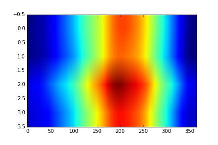

Heatmap of the Data with different aspect ratio

Blue regions in this heat map are low values and red regions high values. As we can see, temperature rises and falls over the year, and the magnitudes are very similar across all four stations.

Let’s take a look at the average temperature between all stations over time:

ave_temp = data.mean(axis=0)
ave_plot = matplotlib.pyplot.plot(ave_temp)
matplotlib.pyplot.show(ave_plot)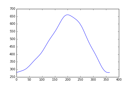

Average Temperature Over Time

It’s interesting to examine how the temperature trends vary between stations throughout the year. We can plot data from each of the stations separately in a single figure using subplots. This script below uses a number of new commands. The function matplotlib.pyplot.figure() creates a space into which we will place all of our plots. The parameter figsize tells Python how big to make this space. Each subplot is placed into the figure using the subplot command. The subplot command takes 3 parameters. The first denotes how many total rows of subplots there are, the second parameter refers to the total number of subplot columns, and the final parameters denotes which subplot your axes name will reference. Each subplot is stored in a different variable (axes1, axes2, axes3, axes4). Once a subplot is created, the axes can be titled using the set_xlabel() or set_ylabel() commands. Here are our four plots stacked:

import numpy as np
import matplotlib.pyplot as plt

data = np.loadtxt(fname='data/temperature.csv', delimiter=',')

fig = plt.figure(figsize=(5.0, 9.0))

axes1 = fig.add_subplot(4, 1, 1)
axes2 = fig.add_subplot(4, 1, 2)
axes3 = fig.add_subplot(4, 1, 3)
axes4 = fig.add_subplot(4, 1, 4)

axes1.set_ylabel('station 0')
axes1.plot(data[0,:])

axes2.set_ylabel('station 1')
axes2.plot(data[1,:])

axes3.set_ylabel('station 2')
axes3.plot(data[2,:])

axes4.set_ylabel('station 3')
axes4.plot(data[3,:])

plt.show(fig)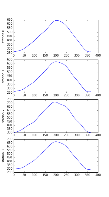

Temperature at each Station as Subplots

When we imported the necessary libraries into this script, we assigned a shortcut or nickname to them (“np” and “plt”) to avoid having to type the full name each time. As before, the call to loadtxt reads our data, and the rest of the program tells the plotting library how large we want the figure to be, that we’re creating four sub-plots, and what to draw for each one.