Programming with Python

Using Pandas with tabular data

At this point, this set of lessons diverges from the usual material included in the Software Carpentry novice Python lessons. The topics we cover are geared towards processing and analyzing scientific data, and handling the complexities that come with pulling data directly from real sources.

We would like to create a script that visualizes the streamgage data from the Colorado River over a specified period of time at different points along its course.

Traditionally, we would access the data through the USGS website, clicking around, dowloading the file, and cleaning it up by hand. The csv file would look like this:

http://waterdata.usgs.gov/az/nwis/uv?cb_00060=on&cb_00065=on&format=rdb&site_no=09380000&period=&begin_date=2016-01-01&end_date=2016-01-10

Instead of cleaning up these files this by hand, we are going to automate the entire process of data import and processing using Python. While manually extracting the data from one file would not take long, repeating the process frequently or with a large number of files would likely lead to errors.

Our code should:

• Take a list of USGS stations, a start date and an end date as input.
• Create plots of the gage height and discharge for each station on the list as output, and save them to individual files.

We will build this script by breaking it up into small tasks, gradually add complexity to our solution, and combine the pieces of code into a single program.

Using Pandas for tabular data

In a previous lesson we used a Python library called NumPy to handle arrays of data. NumPy arrays are perfect for doing calculations with our data, but they can only handle floats or integers. Tabular data more closely resembles spreadsheets, where entries such as dates and times are in some useful format.

One of the best options for working with tabular data in Python is the Python Data Analysis Library (a.k.a. Pandas). The Pandas library provides its own set of data structures, produces high quality plots through Matplotlib (the plotting library we used earlier), and integrates nicely with other libraries that can use NumPy arrays.

Let’s start by importing streamgage data from a file that has already been partially cleaned up. Compare the URL in the introduction with the file we provided: we removed the file header and the column format line (“5d 15s…”), and saved the file as a comma-delimited file instead of tab delimited.

First, we import the Pandas library and give it the shortcut pd. We can use the Pandas function read_csv to import the file and assign them to a variable named data. This will pull the contents of the file into a DataFrame. We can then print the first 5 lines of the DataFrame using the method head():

import pandas as pd

data = pd.read_csv('data/streamgage.csv')
data.head()

Each column in a DataFrame also has a type. We can use data.dtypes to view the data type for each column. int64 represents numeric integer values - int64 cells can not store decimals. object represents strings (letters and numbers). float64 represents numbers with decimals.

data.dtypes

agency_cd       object
site_no          int64
datetime        object
tz_cd           object
01_00060         int64
01_00060_cd     object
02_00065       float64
02_00065_cd     object
dtype: object

We need to give the DataFrame column names that are easier to read. Let’s create a list with the column names we want:

new_column_names = ['Agency', 'Station', 'OldDateTime', 'Timezone', 'Discharge_cfs', 'Discharge_stat', 'Stage_ft', 'Stage_stat']

We can see the column names of a DataFrame using the method columns, and we can use that same method to give the DataFrame the new column names:

print 'Old column names:', data.columns

data.columns = new_column_names

print 'New column names:', data.columns

Old column names: Index([u'agency_cd', u'site_no', u'datetime', u'tz_cd', u'01_00060',
       u'01_00060_cd', u'02_00065', u'02_00065_cd'],
      dtype='object')
New column names: Index([u'Agency', u'Station', u'OldDateTime', u'Timezone', u'Discharge_cfs',
       u'Discharge_stat', u'Stage_ft', u'Stage_stat'],
      dtype='object')

The values in each column of a Pandas DataFrame can be accessed using the column name. If we want to access more than one column at once, we use a list of column names:

data[['Discharge_cfs','Stage_ft']].head()

We can also create new columns using this syntax:

data['Stage_m'] = data['Stage_ft'] * 0.3048

Fixing the station name

When Pandas imported the data, it read the station name as an integer and removed the initial zero. We can fix the station name by replacing the values of that column with a string.

Remember that we are doing all of this so we can later automate the process for multiple stations. Instead of writing the correct station name ourselves, let’s build it from the values available in the DataFrame:

data['Station'].unique()

array([9163500])

The Pandas method unique returns a NumPy array of the unique elements in the Stations column of the DataFrame. We want the first (and only) entry to that array, which has the index 0. We can build a string with the correct station name by casting the integer as a string and concatenating it with an initial zero (also as a string):

new_station_name = "0" + str(data['Station'].unique()[0])
print new_station_name

09163500

We can replace all values in the ‘Station’ column with this string through assignment, and we can check the object type of each column to make sure it is no longer an integer:

data['Station'] = new_station_name
data.dtypes

Agency             object
Station            object
OldDateTime        object
Timezone           object
Discharge_cfs       int64
Discharge_stat     object
Stage_ft          float64
Stage_stat         object
Stage_m           float64
dtype: object

Handling date and time stamps

Different programming languages and software packages handle date and time stamps in their own unique and obscure ways. Pandas has a set of functions for creating and managing timeseries that is well described in the documentation.

We need to convert the entries in the DateTime column into a format that Pandas recognizes. Luckily, the to_datetime function in the Pandas library can convert it directly:

data['DateTime'] = pd.to_datetime(data['OldDateTime'])

Subsetting data and removing columns

The entries in our DataFrame data are indexed by the number in bold on the left side of the row. We can display a slice of the data using index ranges just as we did with NumPy arrays:

data[0:4]

Since we can call individual columns (or lists of columns) from a DataFrame, the simplest way to remove columns is by creating new DataFrames with only the columns we want:

clean_data = data[['Station', 'DateTime', 'Discharge_cfs', 'Stage_ft']]

Plotting stage and discharge

Pandas is well integrated with the Matplotlib library that we used ealier to create plots. We can use the same functions we used before with NumPy arrays or we can use the plotting functions built into Pandas:

import matplotlib.pyplot as plt
%matplotlib inline

plt.plot(data['DateTime'], data['Discharge_cfs'])
plt.title('Station ' + data['Station'][0])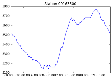

png

data.plot(x='DateTime', y='Discharge_cfs', title='Station ' + data['Station'][0])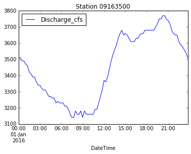

png

We can use pyplot methods to customize the Pandas plot and save the figure:

data.plot(x='DateTime', y='Discharge_cfs', title='Station ' + data['Station'][0])
plt.xlabel('Time')
plt.ylabel('Discharge (cfs)')
plt.show()
plt.savefig('data/discharge_' + data['Station'][0] + '.png')

png

Putting it all together

Let’s go back through the code we’ve written and put together the commands we need to import data and make a plot of discharge:

import pandas as pd
import matplotlib.pyplot as plt
%matplotlib inline

data = pd.read_csv('data/streamgage.csv')

new_column_names = ['Agency', 'Station', 'OldDateTime', 'Timezone', 'Discharge_cfs', 'Discharge_stat', 'Stage_ft', 'Stage_stat']
data.columns = new_column_names

data['DateTime'] = pd.to_datetime(data['OldDateTime'])

new_station_name = "0" + str(data['Station'].unique()[0])
data['Station'] = new_station_name

data.plot(x='DateTime', y='Discharge_cfs', title='Station ' + new_station_name)
plt.xlabel('Time')
plt.ylabel('Discharge (cfs)')
plt.savefig('data/discharge_' + new_station_name + '.png')
plt.show()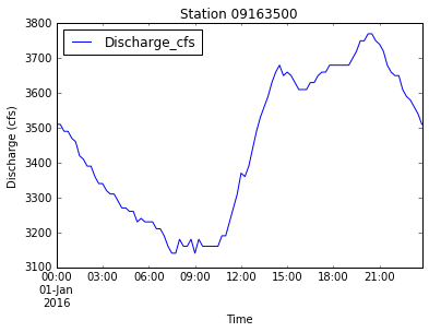

png