Programming with Python

Creating Functions

Learning Objectives

Define a function that takes parameters.
Return a value from a function.
Test and debug a function.
Explain why we should divide programs into small, single-purpose functions.

In the previous two lessons we wrote a script for importing streamgage data through the USGS web services, cleaning up the formatting, plotting the discharge over time, and saving the figure into a file. We would like to turn this script into a tool that we can reuse for different stations and date ranges without having to edit the core of the program. Let’s look at the code again:

import pandas as pd
import matplotlib.pyplot as plt
%matplotlib inline

new_column_names = ['Agency', 'Station', 'OldDateTime', 'Timezone', 'Discharge_cfs', 'Discharge_stat', 'Stage_ft', 'Stage_stat']

url = 'http://waterservices.usgs.gov/nwis/iv/?format=rdb&sites=09380000&startDT=2016-01-01&endDT=2016-01-10&parameterCd=00060,00065'
data = pd.read_csv(url, header=1, sep='\t', comment='#', names = new_column_names)

data['DateTime'] = pd.to_datetime(data['OldDateTime'])

new_station_name = "0" + str(data['Station'].unique()[0])
data['Station'] = new_station_name

data.plot(x='DateTime', y='Discharge_cfs', title='Station ' + new_station_name)
plt.xlabel('Time')
plt.ylabel('Discharge (cfs)')
plt.savefig('data/discharge_' + new_station_name + '.png')
plt.show()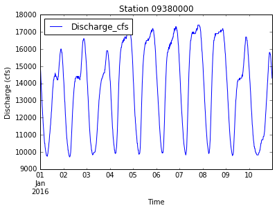

png

The station number and date range we are interested in are part of the URL that we use to communicate with the web services. The specific file we receive when we call the read_csv function doesn’t exist until we request it – when our script calls for some data, the server reads the URL to see what we want, pulls data from a database, packages it into a file, and passes it on to us. The API (the protocol that governs communication between machines) establishes a “formula” for writing the URL, so as long as we follow that formula (and request data that exists), the server will provide it for us.

To understand how it’s built, let’s decompose the URL into parts and combine them back into a single string:

url_root = 'http://waterservices.usgs.gov/nwis/iv/?' # root of URL

url_1 = 'format=' + 'rdb' # file format

url_2 = 'sites=' + '09380000' # station number

url_3 = 'startDT=' + '2016-01-01' # start date

url_4 = 'endDT=' + '2016-01-10' # end date

url_5 = 'parameterCd=' + '00060,00065' # data fields


url = url_root + url_1 + '&' + url_2 + '&' + url_3 + '&' + url_4 + '&' + url_5
print url

  http://waterservices.usgs.gov/nwis/iv/?format=rdb&sites=09380000&startDT=2016-01-01&endDT=2016-01-10&parameterCd=00060,00065

This is not the most elegant way to compose the URL but it accomplishes the job! To clean things up a bit, we can replace the values we want to be able to change with variables:

this_station = '09380000'
startDate = '2016-01-01'
endDate = '2016-01-10'


url_root = 'http://waterservices.usgs.gov/nwis/iv/?'
url_1 = 'format=' + 'rdb'
url_2 = 'sites=' + this_station
url_3 = 'startDT=' + startDate
url_4 = 'endDT=' + endDate
url_5 = 'parameterCd=' + '00060,00065'

url = url_root + url_1 + '&' + url_2 + '&' + url_3 + '&' + url_4 + '&' + url_5
print url

  http://waterservices.usgs.gov/nwis/iv/?format=rdb&sites=09380000&startDT=2016-01-01&endDT=2016-01-10&parameterCd=00060,00065

Python dictionaries to URLs

Another useful data type that is built into Python is the dictionary. While lists and other sequences are indexed by numbers, dictionaries are indexed by keys, so a dictionary is an unordered collection of key:value pairs. Keys must be unique (within any one dictionary) and can be strings or numbers. Values in a dictionary can be of any type, and different keys in one dictionary can be paired with values of different types.

We can store the parameters of the URL in a dictionary. Here’s one of several ways to add entries to a dictionary:

url_dict = {} # create an empty dictionary

url_dict['format'] = 'rdb'
url_dict['sites'] = '09380000'
url_dict['startDT'] = '2016-01-01'
url_dict['endDT'] = '2016-01-10'
url_dict['parameterCd'] = ['00060','00065']

print url_dict

    {'parameterCd': ['00060', '00065'], 'endDT': '2016-01-10', 'startDT': '2016-01-01', 'sites': '09380000', 'format': 'rdb'}

Just like there is the NumPy library for matrices and the Pandas library for tabular data, there is a Python library called urllib that provides a simple interface for accessing resources through URLs (take a look at one package repository for a list of libraries). Many of the most popular and useful libraries for scientific computing come pre-installed with the Anaconda distribution and you can install many more with its package manager conda.

We can use the urllib package to convert the dictionary into a URL following the standard format for APIs:

import urllib

# need to set the parameter doseq to 1 to handle the list in url_dict['parameterCd']
url_parameters = urllib.urlencode(url_dict, doseq=1)

print url_root + url_parameters

   http://waterservices.usgs.gov/nwis/iv/?parameterCd=00060&parameterCd=00065&endDT=2016-01-10&startDT=2016-01-01&sites=09380000&format=rdb

We can now combine it with the rest of our code:

import pandas as pd
import matplotlib.pyplot as plt
%matplotlib inline

########## change these values ###########
this_station = '09380000'
startDate = '2016-01-01'
endDate = '2016-01-10'
##########################################

# create the URL
url_root = 'http://waterservices.usgs.gov/nwis/iv/?'
url_1 = 'format=' + 'rdb'
url_2 = 'sites=' + this_station
url_3 = 'startDT=' + startDate
url_4 = 'endDT=' + endDate
url_5 = 'parameterCd=' + '00060,00065'

url = url_root + url_1 + '&' + url_2 + '&' + url_3 + '&' + url_4 + '&' + url_5

# import the data
new_column_names = ['Agency', 'Station', 'OldDateTime', 'Timezone', 'Discharge_cfs', 'Discharge_stat', 'Stage_ft', 'Stage_stat']

data = pd.read_csv(url, header=1, sep='\t', comment='#', names = new_column_names)

# fix formatting
data['DateTime'] = pd.to_datetime(data['OldDateTime'])
new_station_name = "0" + str(data['Station'].unique()[0])
data['Station'] = new_station_name

# plot and save figure
data.plot(x='DateTime', y='Discharge_cfs', title='Station ' + new_station_name)
plt.xlabel('Time')
plt.ylabel('Discharge (cfs)')
plt.savefig('data/discharge_' + new_station_name + '.png')
plt.show()

png

Creating Functions

If we wanted to import data from a different station or for a different date range using this code, we would manually change the first three variables and run the code again. It would be a lot less work than having to download the file and plot it by hand, but it could still be very tedious! At this point, our code is also getting long and complicated; what if we had thousands of datasets but didn’t want to generate a figure for every single one? Commenting out the figure-drawing code is a nuisance and we might accidentally comment out the wrong lines. Also, what if we want to use that code again, on data with a slightly different format or at a different point in our program? Cutting and pasting code would make it very long and repetitive quickly and probably lead to errors.

We’d like to package our code so that it is easier to reuse. Python provides for this by letting us define things called functions, which create a shorthand way of re-executing longer pieces of code.

As an example, let’s start by defining a function fahr_to_kelvin that converts temperatures from Fahrenheit to Kelvin:

def fahr_to_kelvin(temp):
    return ((temp - 32) * (5/9)) + 273.15

The function definition opens with the word def, followed by the name of the function and a parenthesized list of parameter names. The body of the function — the statements that are executed when the function runs — is indented below the definition, typically by four spaces.

When we call the function, the values we pass to it (the arguments) are assigned to the parameters in the same way that values are assigned to variables. Inside the function, we can use the parameters as variable names that point to the arguments passed to the function. At the end of the body of a function, we can use (but don’t have to) a return statement to send some output to the function call.

Notice that nothing happened when we ran the cell that contains the function. Python became aware of the function as a command that it could run (it became part of the call stack), but nothing will happen until the function is called. Calling our own function is no different from calling any other function:

print 'freezing point of water:', fahr_to_kelvin(32)
print 'boiling point of water:', fahr_to_kelvin(212)

freezing point of water: 273.15
boiling point of water: 273.15

The boiling point of water in Kelvin should be 373.15 K, not 273.15 K!

Functions make code easier to debug by isolating each possible source of error. In this case, we know the error happened inside the function. When we look closely, we can see that the first term of the equation, ((temp - 32) * (5/9)), must be returning 0 (instead of 100) when the temperature is 212 F. If we test each part of that expression, we find:

5/9

5 divided by 9 should be 0.5556, but when we ask Python 2.7 to divide two integers it returns an integer. If we want to keep the fractional part of the division, we need to convert one or the other number to floating point:

print 'two integers:', 5/9
print '5.0/9:', 5.0/9
print '5/9.0:', 5/9.0

two integers: 0
5.0/9: 0.555555555556
5/9.0: 0.555555555556

You can also turn an integer into a float by casting:

float(5)/9

0.5555555555555556

Casting challenges

What happens when you type float(5/9)?

Let’s rewrite our function after fixing the bug:

def fahr_to_kelvin(temp):
    return ((temp - 32) * (5./9)) + 273.15

print 'freezing point of water:', fahr_to_kelvin(32)
print 'boiling point of water:', fahr_to_kelvin(212)

freezing point of water: 273.15
boiling point of water: 373.15

Composing Functions

Now that we’ve seen how to turn Fahrenheit into Kelvin, it’s easy to turn Kelvin into Celsius:

def kelvin_to_celsius(temp_k):
    return temp_k - 273.15

print 'absolute zero in Celsius:', kelvin_to_celsius(0.0)

absolute zero in Celsius: -273.15

What about converting Fahrenheit to Celsius? We could write out the formula but we don’t need to. Instead, we can compose the two functions we have already created:

def fahr_to_celsius(temp_f):
    temp_k = fahr_to_kelvin(temp_f)
    temp_c = kelvin_to_celsius(temp_k)
    return temp_c

print 'freezing point of water in Celsius:', fahr_to_celsius(32.0)

freezing point of water in Celsius: 0.0

This is our first taste of how larger programs are built: we define basic operations and combine them in ever-large chunks to get the effects we want. Real-life functions will usually be larger than the ones shown here — typically half a dozen to a few dozen lines — but they shouldn’t ever be much longer than that or the next person who reads it won’t be able to understand what’s going on.

Combining strings

“Adding” two strings produces their concatenation: 'a' + 'b' is 'ab'. Write a function called fence that takes two parameters called original and wrapper and returns a new string that has the wrapper character at the beginning and end of the original. A call to your function should look like this:

print fence('name', '*')

*name*

Selecting characters from strings

If the variable s refers to a string, then s[0] is the string’s first character and s[-1] is its last. Write a function called outer that returns a string made up of just the first and last characters of its input. A call to your function should look like this:

print outer('helium')

hm

Rescaling an array

Write a function rescale that takes an array as input and returns a corresponding array of values scaled to lie in the range 0.0 to 1.0. (Hint: If L and H are the lowest and highest values in the original array, then the replacement for a value v should be (v − L)/(H − L).)

Variables inside and outside functions

What does the following piece of code display when run - and why?

f = 0
k = 0

def f2k(f):
  k = ((f-32)*(5.0/9.0)) + 273.15
  return k

f2k(8)
f2k(41)
f2k(32)

print k

Tidying up

Now that we know how to wrap bits of code in functions, we can make our code easier to read and easier to reuse. First, let’s make an import_streamgage_data function to pull the data file from the server and fix the formatting:

def import_streamgage_data(url):
    
    new_column_names = ['Agency', 'Station', 'OldDateTime', 'Timezone', 'Discharge_cfs', 'Discharge_stat', 'Stage_ft', 'Stage_stat']

    data = pd.read_csv(url, header=1, sep='\t', comment='#', names = new_column_names)

    # fix formatting
    data['DateTime'] = pd.to_datetime(data['OldDateTime'])
    new_station_name = "0" + str(data['Station'].unique()[0])
    data['Station'] = new_station_name
    
    return data

We can make another function called plot_discharge to plot and save the figures:

def plot_discharge(data):
    
    data.plot(x='DateTime', y='Discharge_cfs', title='Station ' + new_station_name)
    plt.xlabel('Time')
    plt.ylabel('Discharge (cfs)')
    plt.savefig('data/discharge_' + new_station_name + '.png')
    plt.show()

The function plot_discharge produces output that is visible to us (plots and files) but it has no return statement because it doesn’t need to give anything back to the script that called it.

We can also wrap up the script for composing URLs into a function called generate_URL:

def generate_URL(station, startDT, endDT):

    url_root = 'http://waterservices.usgs.gov/nwis/iv/?'
    url_1 = 'format=' + 'rdb'
    url_2 = 'sites=' + station
    url_3 = 'startDT=' + startDT
    url_4 = 'endDT=' + endDT
    url_5 = 'parameterCd=' + '00060,00065'

    url = url_root + url_1 + '&' + url_2 + '&' + url_3 + '&' + url_4 + '&' + url_5
    
    return url

Now that these three functions exist in the call stack, we can rewrite our code as a much simpler script:

########## change these values ###########
this_station = '09380000'
startDate = '2016-01-01'
endDate = '2016-01-10'
##########################################

url = generate_URL(this_station, startDate, endDate)
data = import_streamgage_data(url)
plot_discharge(data)

png

Testing and Documenting

It doesn’t take long to forget what some code we wrote in the past was supposed to do. We should always write some documentation for our functions to remind ourselves (and others) what they do and how they are supposed to be used.

The usual way to put documentation in software is to add comments:

# plot_discharge(data): take a DataFrame containing streamgage data, plot the discharge and save a figure to file.
def plot_discharge(data):
    
    data.plot(x='DateTime', y='Discharge_cfs', title='Station ' + new_station_name)
    plt.xlabel('Time')
    plt.ylabel('Discharge (cfs)')
    plt.savefig('data/discharge_' + new_station_name + '.png')
    plt.show()

It’s easy to misplace comments or make them irrelevant while modifying code, so there’s a better way to document. If the first thing in a function is a string that isn’t assigned to a variable, that string is attached to the function as its documentation. A string like this is called a docstring:

def plot_discharge(data):
    '''
    Take a DataFrame containing streamgage data,
    plot the discharge and save a figure to file.
    '''
    
    data.plot(x='DateTime', y='Discharge_cfs', title='Station ' + new_station_name)
    plt.xlabel('Time')
    plt.ylabel('Discharge (cfs)')
    plt.savefig('data/discharge_' + new_station_name + '.png')
    plt.show()

We can now ask Python’s built-in help system to show us the documentation for the function:

help(plot_discharge)

    Help on function plot_discharge in module __main__:
    
    plot_discharge(data)
        Take a DataFrame containing streamgage data,
        plot the discharge and save a figure to file.

Testing and documenting your function

Run the commands help(numpy.arange) and help(numpy.linspace) to see how to use these functions to generate regularly-spaced values, then use those values to test your rescale function. Once you’ve successfully tested your function, add a docstring that explains what it does.

Defining Defaults:

When we used the read_csv method, we passed parameters in two ways: directly, as in pd.read_csv(url), and by name, as we did for the parameter sep in pd.read_csv(url, sep = '\t').

If we look at the documentation for read_csv, all parameters but the first (filepath_or_buffer) have a default value in the function definition (sep=','). The function will not run if parameters without default values are not provided but all parameters with defaults are optional. This is handy: if we usually want a function to work one way but occasionally need it to do something else, we can allow people to pass a parameter when they need to but provide a default to make the usual case easier.

The example below shows how Python matches values to parameters:

def display(a=1, b=2, c=3):
    print 'a:', a, 'b:', b, 'c:', c 

print 'no parameters:' 
display()

print 'one parameter:'
display(55)

print 'two parameters:'
display(55, 66)

no parameters:
a: 1 b: 2 c: 3
one parameter:
a: 55 b: 2 c: 3
two parameters:
a: 55 b: 66 c: 3

As this example shows, parameters are matched up from left to right and any that haven’t been given a value explicitly get their default value. We can override this behavior by naming the value as we pass it in:

print('only setting the value of c')
display(c=77)

only setting the value of c
a: 1 b: 2 c: 77

Defining defaults

Rewrite the rescale function so that it scales data to lie between 0.0 and 1.0 by default, but will allow the caller to specify lower and upper bounds if they want. Compare your implementation to your neighbor’s: do the two functions always behave the same way?

Grand Challenge!

Turn your code into a function that takes a station number, start date, and end date as arguments.
Write a for loop that passes your new function multiple station names one by one and saves figures for each of them.
Wrap the call to your plotting function in a conditional statement. Add an argument (a boolean - True or False) to the outer function for turning plotting on and off. Give it a default value of True and test calling your function.