Programming with Python

Using Pandas with tabular data

Learning Objectives

Load data using the Pandas library.
Access data in DataFrames.
Create plots of data in DataFrames.
Save figures to file.

By now you have all written some Python code that works so we are going to jump into doing some science tasks with data pulled directly from real sources instead of using a dataset we cleaned for you.

Some of the stuff we are going to do will be fairly advanced but I think that seeing how the language can automate your workflow - and especially how it can handle the tasks that are annoying or difficult - will make it more likely that you’ll come back to it. We are throwing a lot at you, so put a red sticky up if you need hands-on help and interrupt if you have a question, and we’ll adjust as we go.

Streamflow measurements of the Colorado River

We are interested in the comparing the discharge of the Colorado River at different points along its course over a specific time period. The traditional way to do this is through the USGS website:

http://waterwatch.usgs.gov/?m=real&r=az

There we can select, by hand, the specific stations we want and request the data for the period of interest. At the end, we end up with some csv files that look like this:

http://waterdata.usgs.gov/az/nwis/uv?cb_00060=on&cb_00065=on&format=rdb&site_no=09380000&period=&begin_date=2016-01-01&end_date=2016-01-10

The header is difficult to work with because it doesn’t always have the same number of lines. Depending on the options we selected on the website, the table can have a different number of columns. Automating the analysis of these files is complicated and it requires quite a bit of handholding in Excel. If we had to do this frequently or for many stations, the chances that we would introduce an error into the data are high.

Our goal is to automate the entire process of data import and processing using Python. We will write a script that will take two dates and a list of stations and will automatically create plots of the discharge at each of those stations.

Earlier today we used a Python library called NumPy to handle arrays of data. NumPy arrays are great for doing math on data but they can only contain floats or integers. Tabular data are best handled by spreadsheets where entries such as dates and times are in some useful format.

One of the best options for working with tabular data in Python is the Python Data Analysis Library (a.k.a. Pandas). The Pandas library provides data structures for tabular data, produces high quality plots with matplotlib (the plotting library we used earlier) and integrates nicely with other libraries that use NumPy arrays.

Let’s start by importing streamgage data from a file that has already been partially cleaned. Open the file in a text editor and see: we removed the header and the column format line (“5d 15s…”) and saved it as a comma-delimited file instead of tab delimited.

To load this file into Python, we first import the Pandas library and give it the shortcut pd. We can then use the Pandas function read_csv to import the file. This will pull the contents of the file into a DataFrame. Let’s assign it to a variable named data (so original!) and print the first 5 lines:

import pandas as pd

data = pd.read_csv('data/streamgage.csv')
data.head()

<div>
<table border="1" class="dataframe">
  <thead>
    <tr style="text-align: right;">
      <th></th>
      <th>agency_cd</th>
      <th>site_no</th>
      <th>datetime</th>
      <th>tz_cd</th>
      <th>01_00060</th>
      <th>01_00060_cd</th>
      <th>02_00065</th>
      <th>02_00065_cd</th>
    </tr>
  </thead>
  <tbody>
    <tr>
      <th>0</th>
      <td>USGS</td>
      <td>9163500</td>
      <td>1/1/16 0:00</td>
      <td>MST</td>
      <td>3510</td>
      <td>P</td>
      <td>3.78</td>
      <td>P</td>
    </tr>
    <tr>
      <th>1</th>
      <td>USGS</td>
      <td>9163500</td>
      <td>1/1/16 0:15</td>
      <td>MST</td>
      <td>3510</td>
      <td>P</td>
      <td>3.78</td>
      <td>P</td>
    </tr>
    <tr>
      <th>2</th>
      <td>USGS</td>
      <td>9163500</td>
      <td>1/1/16 0:30</td>
      <td>MST</td>
      <td>3490</td>
      <td>P</td>
      <td>3.77</td>
      <td>P</td>
    </tr>
    <tr>
      <th>3</th>
      <td>USGS</td>
      <td>9163500</td>
      <td>1/1/16 0:45</td>
      <td>MST</td>
      <td>3490</td>
      <td>P</td>
      <td>3.77</td>
      <td>P</td>
    </tr>
    <tr>
      <th>4</th>
      <td>USGS</td>
      <td>9163500</td>
      <td>1/1/16 1:00</td>
      <td>MST</td>
      <td>3470</td>
      <td>P</td>
      <td>3.76</td>
      <td>P</td>
    </tr>
  </tbody>
</table>
</div>

print type(data)
print data.__class__

<class 'pandas.core.frame.DataFrame'>
<class 'pandas.core.frame.DataFrame'>

Each column in a DataFrame also has its own type. We can use data.dtypes to view the data type for each column. int64 are numeric integer values - int64 cells can not store decimals, object are strings (letters and numbers), and float64 are numbers with decimals.

data.dtypes

agency_cd       object
site_no          int64
datetime        object
tz_cd           object
01_00060         int64
01_00060_cd     object
02_00065       float64
02_00065_cd     object
dtype: object

We need to give the DataFrame column names that are easier to read. Let’s create a list with the column names we want:

new_column_names = ['Agency', 'Station', 'OldDateTime', 'Timezone', 'Discharge_cfs', 'Discharge_stat', 'Stage_ft', 'Stage_stat']

We can see the column names of a DataFrame using the method columns, and we can use that same method to assign it the new column names:

print 'Old column names:', data.columns

data.columns = new_column_names

print 'New column names:', data.columns

Old column names: Index([u'agency_cd', u'site_no', u'datetime', u'tz_cd', u'01_00060',
       u'01_00060_cd', u'02_00065', u'02_00065_cd'],
      dtype='object')
New column names: Index([u'Agency', u'Station', u'OldDateTime', u'Timezone', u'Discharge_cfs',
       u'Discharge_stat', u'Stage_ft', u'Stage_stat'],
      dtype='object')

data.head()

<div>
<table border="1" class="dataframe">
  <thead>
    <tr style="text-align: right;">
      <th></th>
      <th>Agency</th>
      <th>Station</th>
      <th>OldDateTime</th>
      <th>Timezone</th>
      <th>Discharge_cfs</th>
      <th>Discharge_stat</th>
      <th>Stage_ft</th>
      <th>Stage_stat</th>
    </tr>
  </thead>
  <tbody>
    <tr>
      <th>0</th>
      <td>USGS</td>
      <td>9163500</td>
      <td>1/1/16 0:00</td>
      <td>MST</td>
      <td>3510</td>
      <td>P</td>
      <td>3.78</td>
      <td>P</td>
    </tr>
    <tr>
      <th>1</th>
      <td>USGS</td>
      <td>9163500</td>
      <td>1/1/16 0:15</td>
      <td>MST</td>
      <td>3510</td>
      <td>P</td>
      <td>3.78</td>
      <td>P</td>
    </tr>
    <tr>
      <th>2</th>
      <td>USGS</td>
      <td>9163500</td>
      <td>1/1/16 0:30</td>
      <td>MST</td>
      <td>3490</td>
      <td>P</td>
      <td>3.77</td>
      <td>P</td>
    </tr>
    <tr>
      <th>3</th>
      <td>USGS</td>
      <td>9163500</td>
      <td>1/1/16 0:45</td>
      <td>MST</td>
      <td>3490</td>
      <td>P</td>
      <td>3.77</td>
      <td>P</td>
    </tr>
    <tr>
      <th>4</th>
      <td>USGS</td>
      <td>9163500</td>
      <td>1/1/16 1:00</td>
      <td>MST</td>
      <td>3470</td>
      <td>P</td>
      <td>3.76</td>
      <td>P</td>
    </tr>
  </tbody>
</table>
</div>

The values in each column of a Pandas DataFrame can be accessed using the column name. If we want to access more than one column at once, we use a list of column names:

data[['Discharge_cfs','Stage_ft']].head()

<div>
<table border="1" class="dataframe">
  <thead>
    <tr style="text-align: right;">
      <th></th>
      <th>Discharge_cfs</th>
      <th>Stage_ft</th>
    </tr>
  </thead>
  <tbody>
    <tr>
      <th>0</th>
      <td>3510</td>
      <td>3.78</td>
    </tr>
    <tr>
      <th>1</th>
      <td>3510</td>
      <td>3.78</td>
    </tr>
    <tr>
      <th>2</th>
      <td>3490</td>
      <td>3.77</td>
    </tr>
    <tr>
      <th>3</th>
      <td>3490</td>
      <td>3.77</td>
    </tr>
    <tr>
      <th>4</th>
      <td>3470</td>
      <td>3.76</td>
    </tr>
  </tbody>
</table>
</div>

We can also create new columns using this syntax:

data['Stage_m'] = data['Stage_ft'] * 0.3048
data['Stage_m'].head()

0    1.152144
1    1.152144
2    1.149096
3    1.149096
4    1.146048
Name: Stage_m, dtype: float64

Fixing the station name

When Pandas imported the data, it read the station name (a number) as an integer and removed the initial zero. We can fix the station name by replacing the values of that column with a string.

Remember that the goal is to automate the process for multiple stations. Instead of writing the corrected station name ourselves, let’s build it from the values available in the DataFrame:

data['Station'].unique()

array([9163500])

The Pandas method unique returns a numpy array of the unique elements in the DataFrame. We want the first (and only) entry in that array, which has the index 0. We can build a string with the correct station name by casting that value as a string and concatenating it with an initial zero:

new_station_name = "0" + str(data['Station'].unique()[0])
print new_station_name

09163500

We can replace all values in the ‘Station’ column with this string through assignment and check the object type of each column to make sure it is no longer an integer:

data['Station'] = new_station_name
data.head()

<div>
<table border="1" class="dataframe">
  <thead>
    <tr style="text-align: right;">
      <th></th>
      <th>Agency</th>
      <th>Station</th>
      <th>OldDateTime</th>
      <th>Timezone</th>
      <th>Discharge_cfs</th>
      <th>Discharge_stat</th>
      <th>Stage_ft</th>
      <th>Stage_stat</th>
      <th>Stage_m</th>
    </tr>
  </thead>
  <tbody>
    <tr>
      <th>0</th>
      <td>USGS</td>
      <td>09163500</td>
      <td>1/1/16 0:00</td>
      <td>MST</td>
      <td>3510</td>
      <td>P</td>
      <td>3.78</td>
      <td>P</td>
      <td>1.152144</td>
    </tr>
    <tr>
      <th>1</th>
      <td>USGS</td>
      <td>09163500</td>
      <td>1/1/16 0:15</td>
      <td>MST</td>
      <td>3510</td>
      <td>P</td>
      <td>3.78</td>
      <td>P</td>
      <td>1.152144</td>
    </tr>
    <tr>
      <th>2</th>
      <td>USGS</td>
      <td>09163500</td>
      <td>1/1/16 0:30</td>
      <td>MST</td>
      <td>3490</td>
      <td>P</td>
      <td>3.77</td>
      <td>P</td>
      <td>1.149096</td>
    </tr>
    <tr>
      <th>3</th>
      <td>USGS</td>
      <td>09163500</td>
      <td>1/1/16 0:45</td>
      <td>MST</td>
      <td>3490</td>
      <td>P</td>
      <td>3.77</td>
      <td>P</td>
      <td>1.149096</td>
    </tr>
    <tr>
      <th>4</th>
      <td>USGS</td>
      <td>09163500</td>
      <td>1/1/16 1:00</td>
      <td>MST</td>
      <td>3470</td>
      <td>P</td>
      <td>3.76</td>
      <td>P</td>
      <td>1.146048</td>
    </tr>
  </tbody>
</table>
</div>

data.dtypes

Agency             object
Station            object
OldDateTime        object
Timezone           object
Discharge_cfs       int64
Discharge_stat     object
Stage_ft          float64
Stage_stat         object
Stage_m           float64
dtype: object

Handling date and time stamps

Different programming languages and software packages handle date and time stamps in their own unique and obscure ways. Pandas has a set of functions for creating and managing timeseries that is well described in the documentation.

We need to convert the entries in the DateTime column into a format that Pandas recognizes. Luckily, the to_datetime function in the Pandas library can convert it directly:

data['DateTime'] = pd.to_datetime(data['OldDateTime'])
data.head()

<div>
<table border="1" class="dataframe">
  <thead>
    <tr style="text-align: right;">
      <th></th>
      <th>Agency</th>
      <th>Station</th>
      <th>OldDateTime</th>
      <th>Timezone</th>
      <th>Discharge_cfs</th>
      <th>Discharge_stat</th>
      <th>Stage_ft</th>
      <th>Stage_stat</th>
      <th>Stage_m</th>
      <th>DateTime</th>
    </tr>
  </thead>
  <tbody>
    <tr>
      <th>0</th>
      <td>USGS</td>
      <td>09163500</td>
      <td>1/1/16 0:00</td>
      <td>MST</td>
      <td>3510</td>
      <td>P</td>
      <td>3.78</td>
      <td>P</td>
      <td>1.152144</td>
      <td>2016-01-01 00:00:00</td>
    </tr>
    <tr>
      <th>1</th>
      <td>USGS</td>
      <td>09163500</td>
      <td>1/1/16 0:15</td>
      <td>MST</td>
      <td>3510</td>
      <td>P</td>
      <td>3.78</td>
      <td>P</td>
      <td>1.152144</td>
      <td>2016-01-01 00:15:00</td>
    </tr>
    <tr>
      <th>2</th>
      <td>USGS</td>
      <td>09163500</td>
      <td>1/1/16 0:30</td>
      <td>MST</td>
      <td>3490</td>
      <td>P</td>
      <td>3.77</td>
      <td>P</td>
      <td>1.149096</td>
      <td>2016-01-01 00:30:00</td>
    </tr>
    <tr>
      <th>3</th>
      <td>USGS</td>
      <td>09163500</td>
      <td>1/1/16 0:45</td>
      <td>MST</td>
      <td>3490</td>
      <td>P</td>
      <td>3.77</td>
      <td>P</td>
      <td>1.149096</td>
      <td>2016-01-01 00:45:00</td>
    </tr>
    <tr>
      <th>4</th>
      <td>USGS</td>
      <td>09163500</td>
      <td>1/1/16 1:00</td>
      <td>MST</td>
      <td>3470</td>
      <td>P</td>
      <td>3.76</td>
      <td>P</td>
      <td>1.146048</td>
      <td>2016-01-01 01:00:00</td>
    </tr>
  </tbody>
</table>
</div>

Creating data subsets and removing columns

The entries in our DataFrame data are indexed by the number in bold on the left side of each row. We can display a slice of the data using index ranges:

data[0:4]

<div>
<table border="1" class="dataframe">
  <thead>
    <tr style="text-align: right;">
      <th></th>
      <th>Agency</th>
      <th>Station</th>
      <th>OldDateTime</th>
      <th>Timezone</th>
      <th>Discharge_cfs</th>
      <th>Discharge_stat</th>
      <th>Stage_ft</th>
      <th>Stage_stat</th>
      <th>Stage_m</th>
      <th>DateTime</th>
    </tr>
  </thead>
  <tbody>
    <tr>
      <th>0</th>
      <td>USGS</td>
      <td>09163500</td>
      <td>1/1/16 0:00</td>
      <td>MST</td>
      <td>3510</td>
      <td>P</td>
      <td>3.78</td>
      <td>P</td>
      <td>1.152144</td>
      <td>2016-01-01 00:00:00</td>
    </tr>
    <tr>
      <th>1</th>
      <td>USGS</td>
      <td>09163500</td>
      <td>1/1/16 0:15</td>
      <td>MST</td>
      <td>3510</td>
      <td>P</td>
      <td>3.78</td>
      <td>P</td>
      <td>1.152144</td>
      <td>2016-01-01 00:15:00</td>
    </tr>
    <tr>
      <th>2</th>
      <td>USGS</td>
      <td>09163500</td>
      <td>1/1/16 0:30</td>
      <td>MST</td>
      <td>3490</td>
      <td>P</td>
      <td>3.77</td>
      <td>P</td>
      <td>1.149096</td>
      <td>2016-01-01 00:30:00</td>
    </tr>
    <tr>
      <th>3</th>
      <td>USGS</td>
      <td>09163500</td>
      <td>1/1/16 0:45</td>
      <td>MST</td>
      <td>3490</td>
      <td>P</td>
      <td>3.77</td>
      <td>P</td>
      <td>1.149096</td>
      <td>2016-01-01 00:45:00</td>
    </tr>
  </tbody>
</table>
</div>

`loc` or `iloc`?

Accessing individual rows or subsets of both rows and columns is a bit more obscure. We can select specific ranges of our data in both the row and column directions using either label or integer-based indexing.

loc: indexing via labels or integers
iloc: indexing via integers

To select a subset of rows AND columns from our DataFrame, we can use the iloc method and the integer indices for both rows and columns:

data.iloc[0:2,-2:]

<div>
<table border="1" class="dataframe">
  <thead>
    <tr style="text-align: right;">
      <th></th>
      <th>Stage_m</th>
      <th>DateTime</th>
    </tr>
  </thead>
  <tbody>
    <tr>
      <th>0</th>
      <td>1.152144</td>
      <td>2016-01-01 00:00:00</td>
    </tr>
    <tr>
      <th>1</th>
      <td>1.152144</td>
      <td>2016-01-01 00:15:00</td>
    </tr>
  </tbody>
</table>
</div>

Or the loc method, using integer indices for rows and labels for columns:

data.loc[0:2, ['DateTime', 'Stage_m']]

<div>
<table border="1" class="dataframe">
  <thead>
    <tr style="text-align: right;">
      <th></th>
      <th>DateTime</th>
      <th>Stage_m</th>
    </tr>
  </thead>
  <tbody>
    <tr>
      <th>0</th>
      <td>2016-01-01 00:00:00</td>
      <td>1.152144</td>
    </tr>
    <tr>
      <th>1</th>
      <td>2016-01-01 00:15:00</td>
      <td>1.152144</td>
    </tr>
    <tr>
      <th>2</th>
      <td>2016-01-01 00:30:00</td>
      <td>1.149096</td>
    </tr>
  </tbody>
</table>
</div>

The number of rows that these two commands return is different. The method iloc behaves like slicing elsewhere in Python, ignoring the end bound. With loc, however, the start and end bounds of the row indices are included. Compare them using the shape method:

print 'With iloc:', data.iloc[0:2,-2:].shape
print 'With loc:', data.loc[0:2, ['DateTime', 'Stage_m']].shape

With iloc: (2, 2)
With loc: (3, 2)

Since we can call individual columns (or lists of columns) from a DataFrame, the simplest way to remove columns is by creating a new DataFrame with only the columns we want:

clean_data = data[['Station', 'DateTime', 'Discharge_cfs', 'Stage_ft']]
clean_data.head()

<div>
<table border="1" class="dataframe">
  <thead>
    <tr style="text-align: right;">
      <th></th>
      <th>Station</th>
      <th>DateTime</th>
      <th>Discharge_cfs</th>
      <th>Stage_ft</th>
    </tr>
  </thead>
  <tbody>
    <tr>
      <th>0</th>
      <td>09163500</td>
      <td>2016-01-01 00:00:00</td>
      <td>3510</td>
      <td>3.78</td>
    </tr>
    <tr>
      <th>1</th>
      <td>09163500</td>
      <td>2016-01-01 00:15:00</td>
      <td>3510</td>
      <td>3.78</td>
    </tr>
    <tr>
      <th>2</th>
      <td>09163500</td>
      <td>2016-01-01 00:30:00</td>
      <td>3490</td>
      <td>3.77</td>
    </tr>
    <tr>
      <th>3</th>
      <td>09163500</td>
      <td>2016-01-01 00:45:00</td>
      <td>3490</td>
      <td>3.77</td>
    </tr>
    <tr>
      <th>4</th>
      <td>09163500</td>
      <td>2016-01-01 01:00:00</td>
      <td>3470</td>
      <td>3.76</td>
    </tr>
  </tbody>
</table>
</div>

Plotting stage and discharge

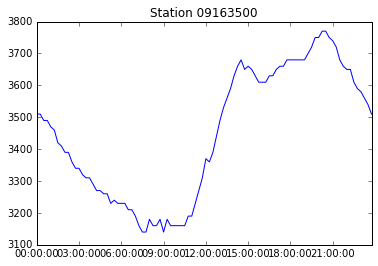
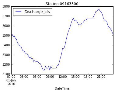
Pandas is well integrated with the matplotlib library that we used ealier in the tutorial. We can either use the same functions we used before with to plot data in NumPy arrays or we can use the plotting functions built into Pandas:

import matplotlib.pyplot as plt
%matplotlib inline

plt.plot(data['DateTime'], data['Discharge_cfs'])
plt.title('Station ' + data['Station'][0])

<matplotlib.text.Text at 0x10a6884d0>
![png](fig/output_37_1.png)

data.plot(x='DateTime', y='Discharge_cfs', title='Station ' + data['Station'][0])

<matplotlib.axes._subplots.AxesSubplot at 0x109eec810>
![png](fig/output_38_1.png)

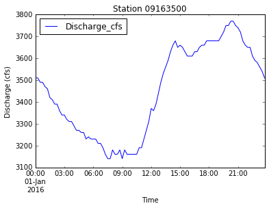
We can use pyplot commands to customize the Pandas plot and save the figure:

data.plot(x='DateTime', y='Discharge_cfs', title='Station ' + data['Station'][0])
plt.xlabel('Time')
plt.ylabel('Discharge (cfs)')
plt.show()
plt.savefig('data/discharge_' + data['Station'][0] + '.png')

![png](fig/output_40_0.png)
<matplotlib.figure.Figure at 0x10b205890>

Putting it all together

Let’s go back through the code we’ve written and put together just the commands we need to import data and make a plot of discharge.

import pandas as pd
import matplotlib.pyplot as plt
%matplotlib inline

data = pd.read_csv('data/streamgage.csv')

new_column_names = ['Agency', 'Station', 'OldDateTime', 'Timezone', 'Discharge_cfs', 'Discharge_stat', 'Stage_ft', 'Stage_stat']
data.columns = new_column_names

data['DateTime'] = pd.to_datetime(data['OldDateTime'])

new_station_name = "0" + str(data['Station'].unique()[0])
data['Station'] = new_station_name

data.plot(x='DateTime', y='Discharge_cfs', title='Station ' + new_station_name)
plt.xlabel('Time')
plt.ylabel('Discharge (cfs)')
plt.savefig('data/discharge_' + new_station_name + '.png')
plt.show()

![png](fig/output_42_0.png)