Programming with Python

Merging DataSets in pandas

In many “real world” situations, the data that we want to use come in multiple files. We often need to combine these files into a single DataFrame to analyze the data. The pandas package provides various methods for combining DataFrames including merge and concat.

To work through the examples below, we first need to load the species and surveys files into pandas DataFrames. In iPython:

import pandas as pd
surveys_df = pd.read_csv('data/surveys.csv', keep_default_na=False, na_values=[""])
surveys_df

       record_id  month  day  year  plot species  sex  wgt
0              1      7   16  1977     2      NA    M  NaN
1              2      7   16  1977     3      NA    M  NaN
2              3      7   16  1977     2      DM    F  NaN
3              4      7   16  1977     7      DM    M  NaN
4              5      7   16  1977     3      DM    M  NaN
...          ...    ...  ...   ...   ...     ...  ...  ...
35544      35545     12   31  2002    15      AH  NaN  NaN
35545      35546     12   31  2002    15      AH  NaN  NaN
35546      35547     12   31  2002    10      RM    F   14
35547      35548     12   31  2002     7      DO    M   51
35548      35549     12   31  2002     5     NaN  NaN  NaN

[35549 rows x 8 columns]

species_df = pd.read_csv('data/species.csv', keep_default_na=False, na_values=[""])
species_df

   species_id             genus          species                   taxa
0          AB        Amphispiza        bilineata                   Bird
1          AH  Ammospermophilus          harrisi    Rodent-not censused
2          AS        Ammodramus       savannarum                   Bird
3          BA           Baiomys          taylori                 Rodent
4          CB   Campylorhynchus  brunneicapillus                   Bird
..        ...               ...              ...                    ...
50         UR            Rodent              sp.                 Rodent
51         US           Sparrow              sp.                   Bird
52         XX               NaN              NaN  Zero Trapping Success
53         ZL       Zonotrichia       leucophrys                   Bird
54         ZM           Zenaida         macroura                   Bird

[55 rows x 4 columns]

Take note that the read_csv method we used can take some additional options which we didn’t use previously. Many functions in python have a set of options that can be set by the user if needed. In this case, we have told Pandas to assign empty values in our CSV to NaN keep_default_na=False, na_values=[""]. http://pandas.pydata.org/pandas-docs/dev/generated/pandas.io.parsers.read_csv.html

Concatenating DataFrames

We can use the concat function in Pandas to append either columns or rows from one DataFrame to another. Let’s grab two subsets of our data to see how this works.

# read in first 10 lines of surveys table
surveySub = surveys_df.head(10)
# grab the last 10 rows (minus the last one)
surveySubLast10 = surveys_df[-11:-1]
#reset the index values to the second dataframe appends properly
surveySubLast10=surveySubLast10.reset_index()

When we concatenate DataFrames, we need to specify the axis. axis=0 tells Pandas to stack the second DataFrame under the first one. It will automatically detect whether the column names are the same and will stack accordingly. axis=0 will stack the columns in the second DataFrame to the RIGHT of the first DataFrame. To stack the data vertically, we need to make sure we have the same columns and associated column format in both datasets. When we stack horizonally, we want to make sure what we are doing makes sense (ie the data are related in some way).

# stack the DataFrames on top of each other
verticalStack = pd.concat([surveySub, surveySubLast10], axis=0)

# place the DataFrames side by side
horizontalStack = pd.concat([surveySub, surveySubLast10], axis=1)

Row Index Values and Concat

Have a look at the horizontalStack DataFrame you just created. Notice anything unusual? The row indexes for the two data frames surveySub and surveySubLast10 are not the same. Thus, when Python tries to concatenate the two dataframes it can’t place them next to each other. We can reindex our second dataframe using the reset_index() method.

```python #reindex the data and then run concat again

surveySubLast10 = surveysSubLast10.reset_index() horizontalStack = pd.concat([surveySub, surveySubLast10], axis=1) ```

The new horizontalStack DataFrame is now side by side without the extra NaN values.

Writing out your data

When you are finished merging your DataFrames, you might want to export the data for future use. We can use the to_csv command to do this. Note that the code below will by default save the data into the current working directory. We could save it to a different folder by adding the foldername and a slash to the file verticalStack.to_csv('foldername/out.csv').

# Write DataFrame to CSV 
verticalStack.to_csv('out.csv')

Check out your working directory to make sure the CSV wrote out properly, and that you can open it! If you want, try to bring it back into python to make sure it imports properly.

# for kicks read our output back into python and make sure all looks good
newOutput = pd.read_csv('out.csv', keep_default_na=False, na_values=[""])

Joining DataFrames

When we concatenated our DataFrames we simply glued them to each other - stacking them either vertically or side by side. Another way to combine DataFrames is to combine them using columns in each dataset that contain common values (a common unique id) as a guide. Combining DataFrames using a common field is called “joining”. The columns containing the common values are called “join key(s)”. Joining DataFrames in this way is often useful when one DataFrame is a “lookup table” containing additional data that we want to include in the other.

NOTE: This process of joining tables is similar to what we do with tables in an SQL database.

For example, the species.csv file that we’ve been working with is a lookup table. This table contains the genus, species and taxa code for 55 species. The species code is unique for each line. These species are identified in our survey data as well using the unique species code. Rather than adding 3 more columns for the genus, species and taxa to each of the 35,549 line Survey data table, we can maintain the shorter table with the species information. When we want to access that information, we can create a query that joins the additional columns of information to the survey data.

Joining two DataFrames

To better understand joins, let’s grab the first 10 lines of our data as a subset to work with. We’ll use the .head method to do this. We’ll also read in a subset of the species table.

# read in first 10 lines of surveys table
surveySub = surveys_df.head(10)

# import a small subset of the species data designed for this part of the lesson
speciesSub = pd.read_csv('speciesSubset.csv', keep_default_na=False, na_values=[""])

In this example, speciesSub is the lookup table containing genus, species, and taxa names that we want to join with the data in surveySub to produce a new DataFrame that contains all of the columns from both species_df and survey_df.

Identifying join keys

To identify appropriate join keys we first need to know which field(s) are shared between the files (DataFrames). We might inspect both DataFrames to identify these columns. If we are lucky, both DataFrames will have columns with the same name that also contain the same data. If we are less lucky, we need to identify a (differently-named) column in each DataFrame that contains the same information.

speciesSub.columns

Index([u'species_id', u'genus', u'species', u'taxa'], dtype='object')

surveySub.columns

Index([u'record_id', u'month', u'day', u'year', u'plot', u'species', u'sex', u'wgt'], dtype='object')

In our example, the join key is the column containing the two-letter species identifier, which is called species in surveys_df and species_id in species_df.

Now that we know the fields with the common species ID attributes in each DataFrame, we are almost ready to join our data. However, since there are different types of joins, we also need to decide which type of join makes sense for our analysis.

Inner joins

The most common type of join is called an inner join. An inner join combines two DataFrames based on a join key and returns a new DataFrame that contains only those rows that have matching values in both of the original DataFrames.

Inner joins yield a DataFrame that contains only rows where the value being joins exists in BOTH tables. An example of an inner join, adapted from this page is below:

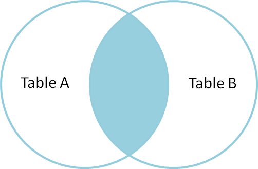
Inner join – courtesy of codinghorror.com

The pandas function for performing joins is called merge and an Inner join is the default option:

merged_inner = pd.merge(left=surveySub,right=speciesSub, left_on='species', right_on='species_id')

merged_inner

    record_id   month   day     year    plot    species_x   sex     wgt     species_id  genus   species_y   taxa
2   3   7   16  1977    2   DM  F   NaN     DM  Dipodomys   merriami    Rodent
3   4   7   16  1977    7   DM  M   NaN     DM  Dipodomys   merriami    Rodent
4   5   7   16  1977    3   DM  M   NaN     DM  Dipodomys   merriami    Rodent
5   8   7   16  1977    1   DM  M   NaN     DM  Dipodomys   merriami    Rodent
6   9   7   16  1977    1   DM  F   NaN     DM  Dipodomys   merriami    Rodent
7   7   7   16  1977    2   PE  F   NaN     PE  Peromyscus  eremicus    Rodent

The result of an inner join of surveySub and speciesSub is a new DataFrame that contains the combined set of columns from surveySub and speciesSub. It only contains rows that have two-letter species codes that are the same in both the surveysSub and speciesSub DataFrames. In other words, if a row in surveySub has a value of species that does not appear in the species_id column of species, it will not be included in the DataFrame returned by an inner join. Similarly, if a row in speciesSub has a value of species_id that does not appear in the species column of surveySub, that row will not be included in the DataFrame returned by an inner join.

The two DataFrames that we want to join are passed to the merge function using the left and right argument. The left_on='species' argument tells merge to use the species column as the join key from surveySub (the left DataFrame). Similarly , the right_on='species_id' argument tells merge to use the species_id column as the join key from speciesSub (the right DataFrame). For inner joins, the order of the left and right arguments does not matter.

The result merged_inner DataFrame contains all of the columns from surveySub (record id, month, day, etc.) as well as all the columns from speciesSub (species id, genus, species, and taxa). Because both original DataFrames contain a column named species, pandas automatically appends a _x to the column name from the left DataFrame and a _y to the column name from the right DataFrame.

Notice that merged_inner has fewer rows than surveysSub. This is an indication that there were rows in surveys_df with value(s) for species that do not exist as value(s) for species_id in species_df.

Left joins

What if we want to add information from speciesSub to surveysSub without losing any of the information from surveySub? In this case, we use a different type of join called a “left outer join”, or a “left join”.

Like an inner join, a left join uses join keys to combine two DataFrames. Unlike an inner join, a left join will return all of the rows from the left DataFrame, even those rows whose join key(s) do not have values in the right DataFrame. Rows in the left DataFrame that are missing values for the join key(s) in the right DataFrame will simply have null (i.e., NaN or None) values for those columns in the resulting joined DataFrame.

Note: a left join will still discard rows from the right DataFrame that do not have values for the join key(s) in the left DataFrame.

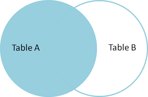
Left Join

A left join is performed in pandas by calling the same merge function used for inner join, but using the how='left' argument:

merged_left = pd.merge(left=surveySub,right=speciesSub, how='left', left_on='species', right_on='species_id')

merged_left

    record_id   month   day     year    plot    species_x   sex     wgt     species_id  genus   species_y   taxa
0   1   7   16  1977    2   NL  M   NaN     NL  Neotoma     albigula    Rodent
1   2   7   16  1977    3   NL  M   NaN     NL  Neotoma     albigula    Rodent
2   3   7   16  1977    2   DM  F   NaN     DM  Dipodomys   merriami    Rodent
3   4   7   16  1977    7   DM  M   NaN     DM  Dipodomys   merriami    Rodent
4   5   7   16  1977    3   DM  M   NaN     DM  Dipodomys   merriami    Rodent
5   8   7   16  1977    1   DM  M   NaN     DM  Dipodomys   merriami    Rodent
6   9   7   16  1977    1   DM  F   NaN     DM  Dipodomys   merriami    Rodent
7   6   7   16  1977    1   PF  M   NaN     NaN     NaN     NaN     NaN
8   10  7   16  1977    6   PF  F   NaN     NaN     NaN     NaN     NaN
9   7   7   16  1977    2   PE  F   NaN     PE  Peromyscus  eremicus    Rodent

The result DataFrame from a left join (merged_left) looks very much like the result DataFrame from an inner join (merged_inner) in terms of the columns it contains. However, unlike merged_inner, merged_left contains the same number of rows as the original surveysSub DataFrame. When we inspect merged_left, we find there are rows where the information that should have come from speciesSub (i.e., species_id, genus, species_y, and taxa) is missing (they contain NaN values):

merged_left[ pd.isnull(merged_left.species_id) ]

    record_id   month   day     year    plot    species_x   sex     wgt     species_id  genus   species_y   taxa
7   6   7   16  1977    1   PF  M   NaN     NaN     NaN     NaN     NaN
8   10  7   16  1977    6   PF  F   NaN     NaN     NaN     NaN     NaN

These rows are the ones where the value of species from surveySub (in this case, NaN) does not occur in speciesSub.